EOQ Essentials: EOQ, Safety Stock, Reorder Points, and More.

---

EOQ Essentials: EOQ, Safety Stock, Reorder Points, and More.

Data Mastery Series — Episode 16: The Art of EOQ (Part 2)

Connect with me and follow our journey: linkedin.com/in/nattapong-thanngam

---

As we delve deeper into supply chain insights, here’s a quick review of our series so far:

• EP1 Time Series Basics:Explored main forecasting methods and evaluated key metrics.
• EP2 Descriptive Analytics I:Discussed the importance of past data and how to visualize it.
• EP3 Descriptive Analytics II: Covered centrality, variability, and localization metrics and introduced handy Python tools for data work.
• EP4 Forecasting Visuals: Showcased line charts and other visuals for time series data.
• EP5 Sales Predictions: Summarized top methods for forecasting sales.
• EP6 EOQ Fundamentals: Introduced the foundations of Economic Order Quantity, focusing on optimizing inventory and reducing costs.

Continuing our Tale

After implementing basic EOQ in her coffee shop business, Zara quickly recognized its limitations, particularly assumptions like constant demand and instantaneous receipt of materials. Seeking more advanced insights, she consulted Donato to explore the nuances of EOQ further.

Put yourself in Zara’s position. What more would you need to know? How can you realistically apply EOQ in a business where demand and lead times are unpredictable? In this episode, we’ll delve into EOQ adaptations for varying demand, dynamic lead times, safety stock (SS), and reorder points (ROP).

---

Figure: Overview of a Simplified Supply Chain Process (Image by Author)

In episodes EP1 through EP5 of “Time Series Forecasting,” we centered on the customer-facing side of the “Coffee Cafe.” Now, just like in EP6, we shift our focus to the supply side, exploring the journey from the “Roasting Facility” to the “Coffee Cafe.”

Understanding EOQ and Its Assumptions

The Economic Order Quantity (EOQ) is calculated using the formula: EOQ = √(2 * D * S / H). Key assumptions here are that the demand is steady and known, and that materials are instantly replenished, indicating a zero lead time.

Diving Deeper: Reorder Points, Safety Stock, and Lead Time:

• Reorder Point (ROP): It signifies the level at which new inventory should be ordered to avoid stockouts. The formula is:
  ROP = (Average Daily Demand × Lead Time) + Safety Stock
• Safety Stock (SS): A protective buffer against unforeseen demand spikes or supply disruptions. Its calculation often accounts for both lead time and demand variability:
  SS=Z×√{(Standard Deviation of Demand² ×Average Lead Time) +(Average Demand² × Standard Deviation of Lead Time²)​}
• Lead Time: The duration between placing an order and receiving it. Illustrated below is a graph depicting a variable lead time, typically ranging from 2–3 days.

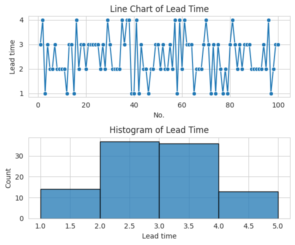
Figure: Simulated Lead Time (Image by Author)

Step 1: Using the Same Dataset from EP6

The dataset simulates 4 SKUs (A-D), each demonstrating distinct demand patterns:

• SKU-A has an increasing trend with seasonality.
• SKU-B shows a decline trend with seasonality.
• SKU-C moves sideways with seasonality.
• SKU-D exhibits random, abrupt spikes in demand.

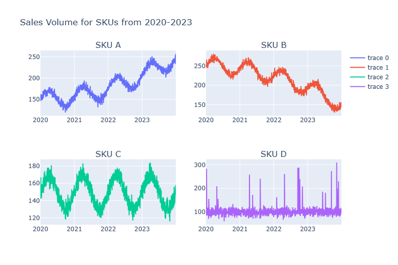
Figure: Sales Trends for SKUs A, B, C, and D from 2020–2023 (Image by Author)

Step 2: Parameter Calculation

While EP5 covered parameters from index 0–9, to determine ROP and SS, we need to delve deeper. This involves computations for average demand, standard deviation of demand, average lead time (rounded up for simplicity), lead time’s standard deviation, and an assumed customer service level (95%). The below table presents these results.

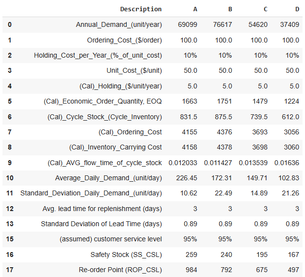
Figure: Calculation Table for SKU A, B, C and D (Image by Author)

Step 3: Tracking Inventory Movements

Using a similar table layout as in EP5, The inventory pattern for SKUs A, B, C, and D has been shown.

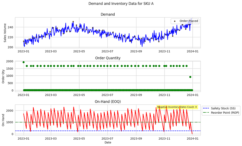
Figure: Inventory Trend with Standard EOQ for SKU A (Image by Author)

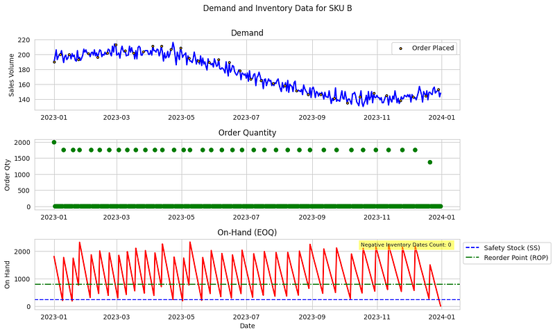
Figure: Inventory Trend with Standard EOQ for SKU B (Image by Author)

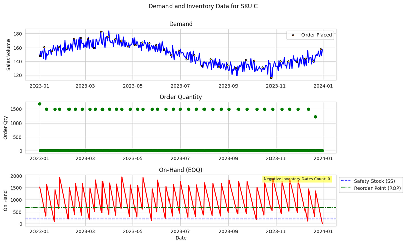
Figure: Inventory Trend with Standard EOQ for SKU C (Image by Author)

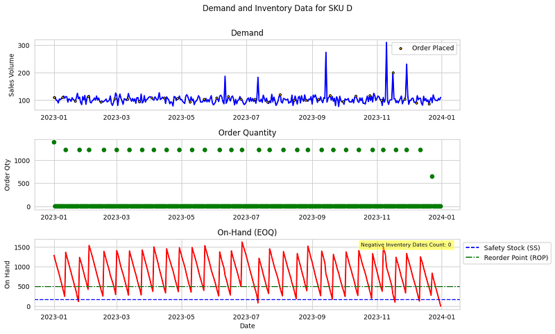
Figure: Inventory Trend with Standard EOQ for SKU D (Image by Author)

Though these charts exhibit the baseline EOQ approach, real-world applications of EOQ offer more sophisticated techniques to further optimize costs. Some of these include:

• Periodic EOQ Ordering: A method where reorders occur at fixed intervals. Here’s a sample of its impact:

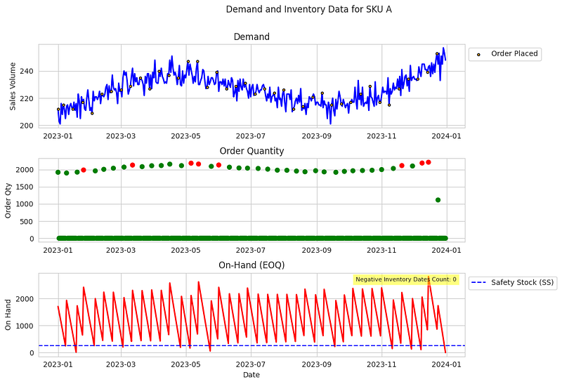
Figure: Periodic EOQ Inventory Trend for SKU A (Image by Author)

• Silver Meal Technique: An approach designed for cost minimization over periods. Sample output follows:

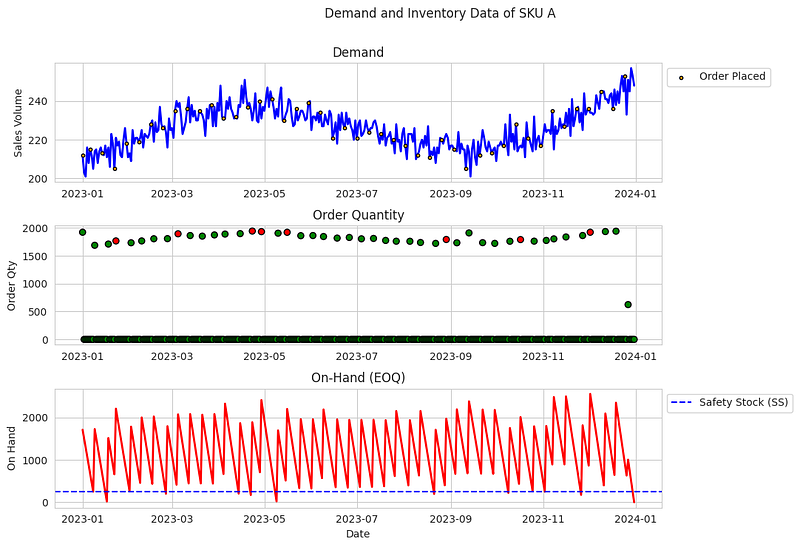
Figure: Silver Meal Inventory Trend for SKU A (Image by Author)

Additionally, there are other EOQ variants suited for different scenarios, such as multi-product EOQ, unit discount EOQ, step discount EOQ, and one-time discount EOQ, each of which finds its application in various business setups.

Concluding Notes

Navigating the complexities of inventory management requires not just theoretical knowledge but also a hands-on understanding of various tools and techniques. This exploration into EOQ and its many facets is a testament to the importance of melding theory with practice. As with all business strategies, adaptability and continual learning are key. I invite you to remain curious, challenge assumptions, and always strive for optimization. Let this series be a starting point, not an end, in your supply chain mastery journey.

Thank you for your engagement and trust throughout this exploration. I look forward to sharing more insights and learnings with you in the future. Until next time, happy optimizing!

---

Data Science Explore the world of data science with Donato_Story

Dashboard Discover the power of data visualization with Donato_Story

Donato_Journey Join me on my journey (Thai version)

Course_Review Discover the training courses with Donato_Story (Thai version)

Please feel free to contact me. I am willing to share and exchange ideas on topics related to data science and supply chains. Medium: medium.com/donato-story
Facebook: web.facebook.com/DonatoStory
Linkedin: linkedin.com/in/nattapong-thanngam