Time Series Forecasting with Python (Part 3)
ARIMA and Prophet by Python
If you are interested in articles related to my experience, please feel free to contact me: linkedin.com/in/nattapong-thanngam
This article is part of a series about Customer Analytics_._ (Part 1: Basic Time Series Forecasting with R),(Part 2: ETS, ARIMA, and Prophet Method by R_)_, (Part 3: ARIMA and Prophet Method by Python_)_
Overview:
- Data source name: Monthly CO2 Concentration (ppm) at Hawaii
- Program: Python
- I do not say which one is better (R vs Python) or (ETS, ARIMA, Prophet). I think different data set will get different result.
This article only shows guidelines for comparison that we can use for our forecasting. - I select RMSE (validation period) to compare model performance
ARIMA by Python (Grid Search)
- I found 3 technics that consist of
- import statsmodels.api as sm
- import pmdarima
from pmdarima.arima import auto_arima - from sktime.forecasting.arima import AutoARIMA
1) import statsmodels.api as sm
- Thank you K.Jessica Forrest-Baldini. I learn all code from her.
- Step of coding same as part 1 & 2
- Base on “import statsmodels.api as sm” and Set Grid search as
- p = q = [0,3]
- d = [0,2] - Grid Search Result:
- Select ARIMA model (3, 1, 0) x (3, 1, 2, 12)12
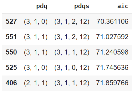
Grid Search Result (Image by Author)
- Result:
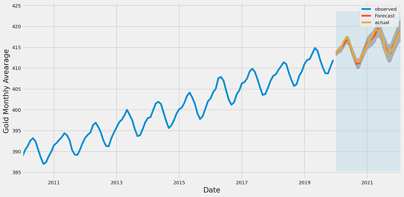
- RMSE = 0.3876 and residual plot is ok.
Predicted value vs Actual data (Image by Author)
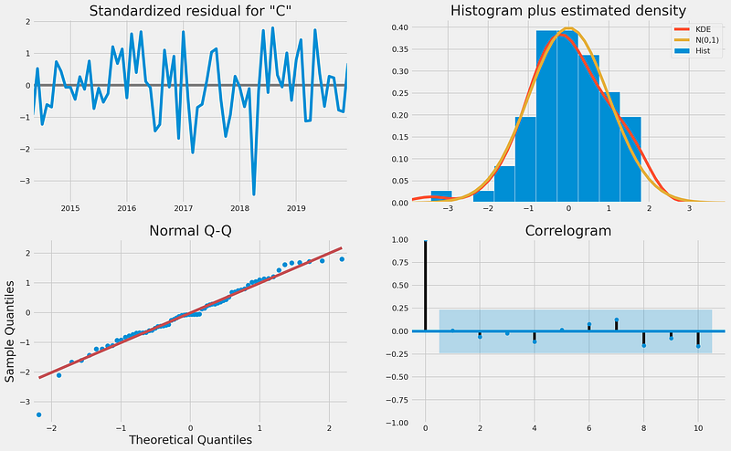
Residual plot by ARIMA model (Image by Author)
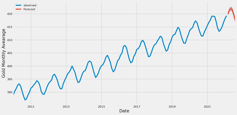
FCST data by ARIMA model (Image by Author)
2) import pmdarima
- Step of coding same as part 1 & 2.
However, this method has to Test for Stationarity.
If adf_test value < 0.05, it means non-stationary.
from pmdarima.arima import ADFTest
adf_test = ADFTest(alpha = 0.05)
adf_test.should_diff(y1)
- Based on “from pmdarima.arima import auto_arima” with the following set up
auto_model = auto_arima(y1,start_p=0, d=1, start_q=0,
max_p=3, max_d=2, max_q=3,
start_P=0, D=1, start_Q=0,
max_P=3, max_D=2, max_Q=3,m=12,
error_action='warn',trace = True,
supress_warnings=True, random_state=20)
- Grid Search Result:
- Best model: ARIMA(0,1,1)(3,1,0)[12]
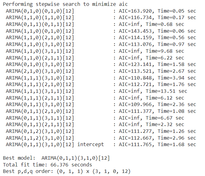
Grid Search Result (Image by Author)
- Result:
- RMSE = 0.2928 and residual plot is ok.
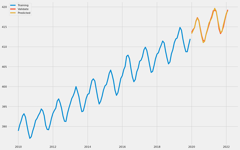
Predicted value vs Actual data (Image by Author)
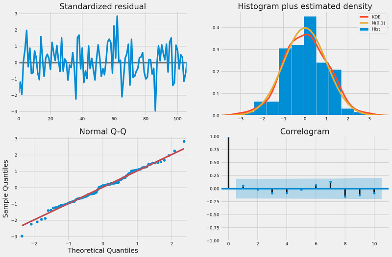
Residual plot by ARIMA model (Image by Author)
3) from sktime.forecasting.arima import AutoARIMA
- Step of coding same as part 1 & 2.
- Based on “from sktime.forecasting.arima import AutoARIMA” with the following set up
forecaster = AutoARIMA(start_p=0, max_p=3, sp=12, seasonal=True, suppress_warnings=True)
- Grid Search Result:
- Best model: SARIMAX(2, 0, 0)x(2, 1, 0, 12)
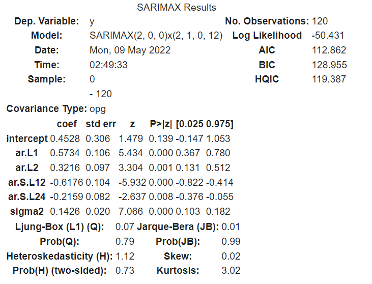
Grid Search Result (Image by Author)
- Result:
- RMSE = 0.4081
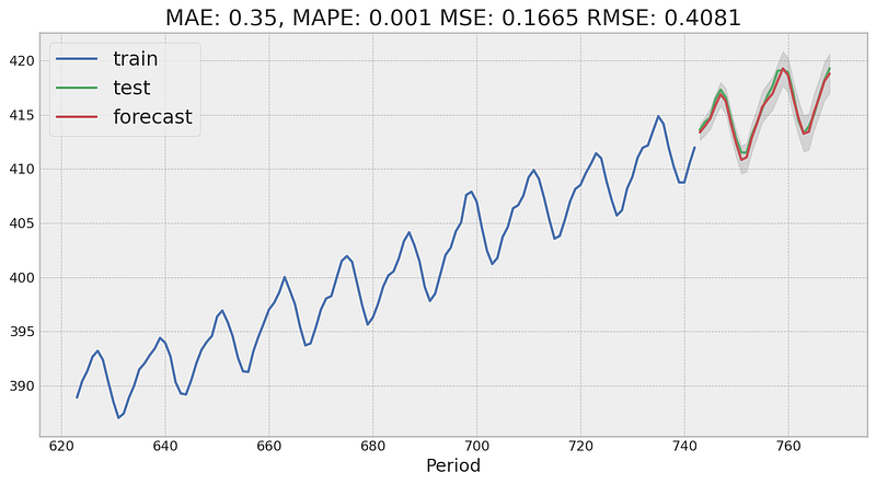
Predicted value vs Actual data (Image by Author)
Prophet by Python
- Step of coding same as part 1 or 2
- Result:
- RMSE = 0.6292
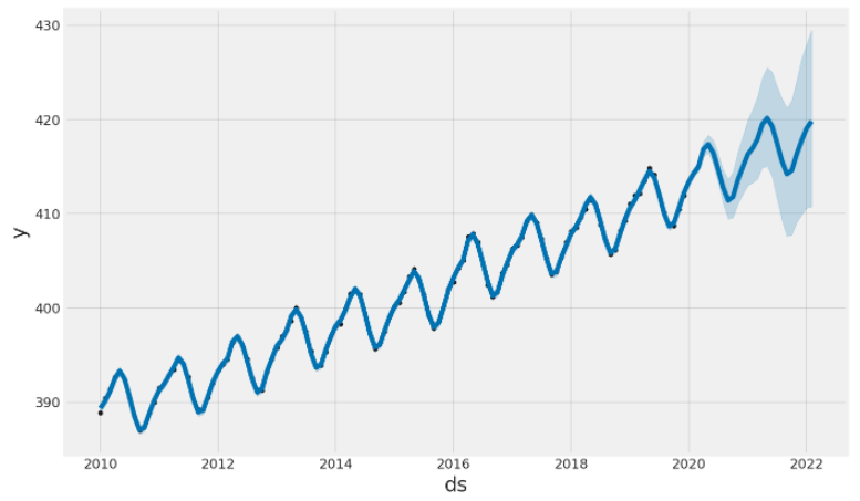
Predicted value vs Actual data (Image by Author)
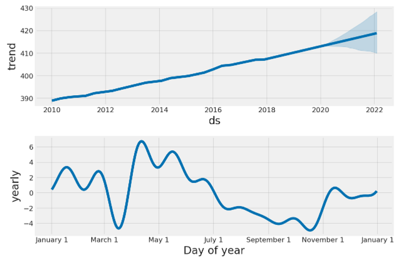
Trend and Season (Image by Author)
Note:
- Summary of all model results.
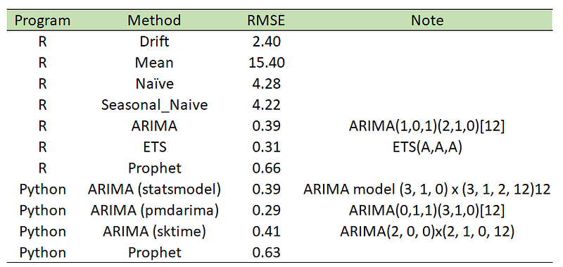
- Again. I think different data set will get different result. I only recommend the step of model comparison.
Please feel free to contact me, I am willing to share and exchange on topics related to Data Science and Supply Chain.
Facebook: facebook.com/nattapong.thanngam
Linkedin: linkedin.com/in/nattapong-thanngam