Framework of income predicting

---

Framework of income predicting

Binary classification, “Adult-income” data set

If you are interested in articles related to my experience, please feel free to contact me: linkedin.com/in/nattapong-thanngam

---

Data source overview:

• Data source name: Adult Data Set
• Abstract: Predict whether income exceeds $50K/yr based on census data. Also known as “Census Income” dataset
• 48,842 data points + 14 features (Age, Workclass, Marital-status, Occupation, Sex, Capital gain/loss, etc.)

Step 1) Split data to Train/Test

• Example of raw data

Raw Data (Image by Author)

• Actually, we do not know the result at the beginning period. Therefore, I think it will be better to separate Train/Test first.

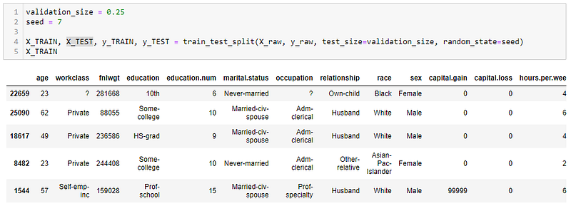
Train/Test split (Image by Author)

Step 2) Data visualization

• Correlation heatmap

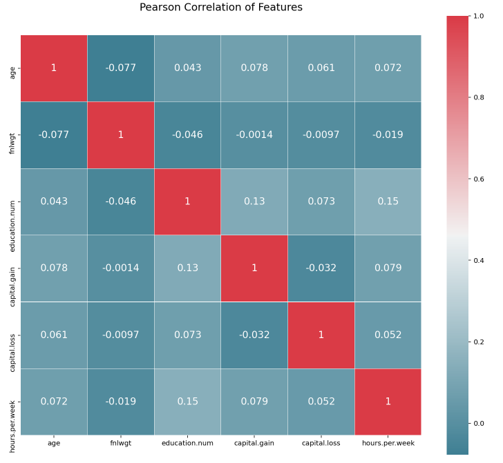
Correlation heatmap (Image by Author)

– Understand predictive relationship between response and predictor variables. In case there is strong positive or negative correlation, the predictor variables can be considered as features for training the models.
– Understand the linear relationship between predictor variables to determine multicollinearity. If the correlation between predictor variables comes out to be greater than 0.7 or less than -0.7, one of these variables can be removed as predictor variable when training the model. In presence of predictor variables having multicollinearity, the coefficients of the predictor variables in the model can be unreliable.

• Overview all data

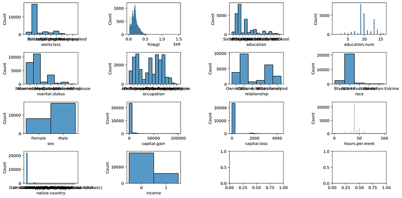
Histogram plot (Image by Author)

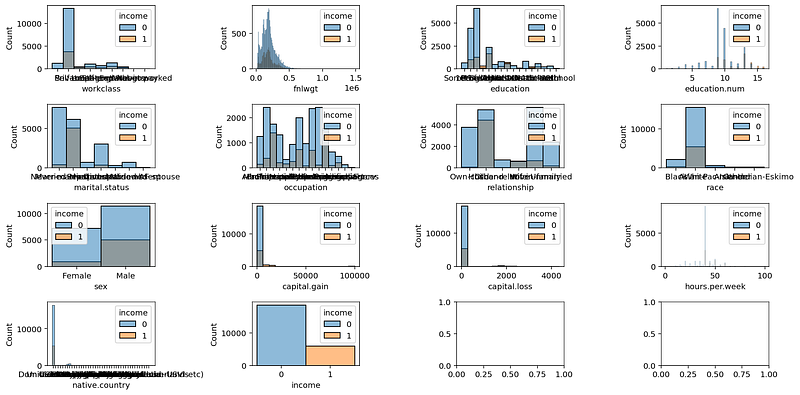
Histogram plot with class (Image by Author)

• We will have more data understanding when we see the graph

Step 3) Data labeling

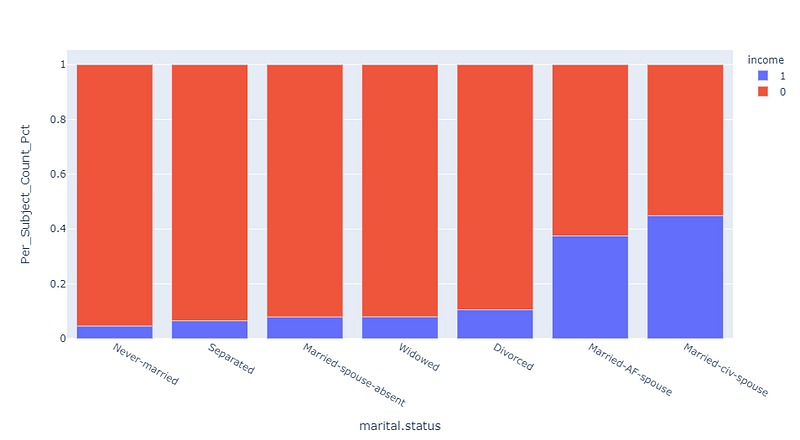
Percentage of 0–1 based on marital status (Image by Author)

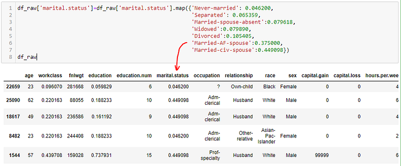
Data Labeling (Image by Author)

• I try a new way for data labeling by using percentage of each parameter.

Step 4) Feature Selection

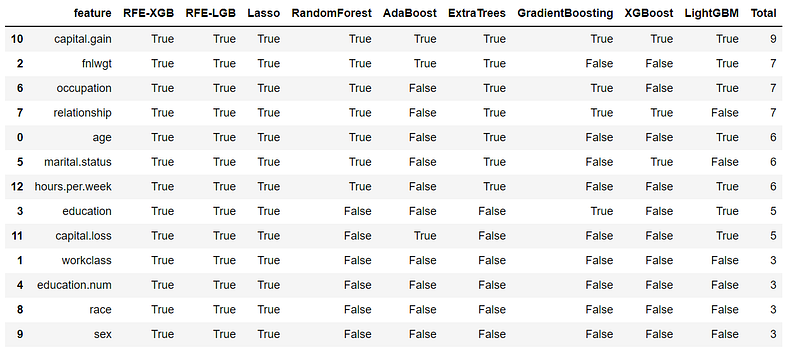
Select feature by voting (Image by Author)

• I select features that have vote score higher than 4 as “X_selection”
• However, I still keep all feature as “X_original”

Step 5) Model comparison

• For this project, I compare 7 algorithm (DecisionTree, LogisticRegression, kNN, RandomForest, XGBoost, LightGBM, GradientBoostingClassifier)
• I use 9 resampling model (no resampler, undersampler, oversampler, smote, smote_tomek, smote_svm, smote_enn, smote_borderline, adasyn)
• I use “StratifiedKFold” function by set “n_splits = 5”
• Ranking by “Average score of AUC”

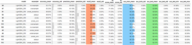
Ranking table (Image by Author)

Step 6) Model tuning

• After tuning, the AUC score increased from 92.69% to 92.90%

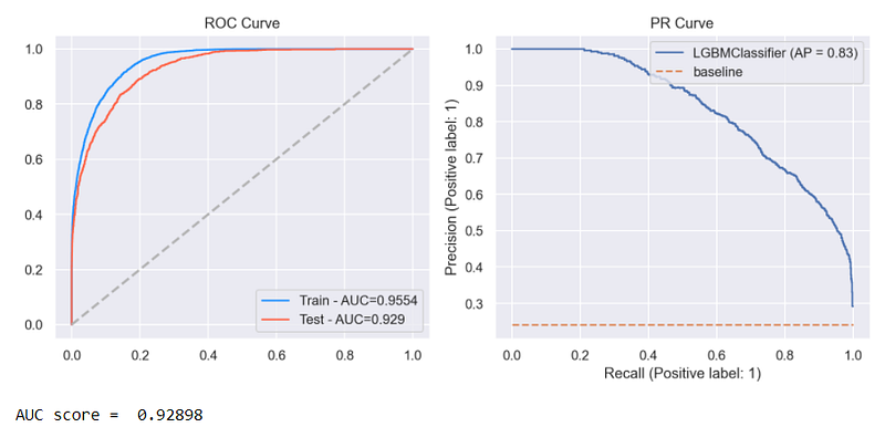
ROC curve after tuning (Image by Author)

Summary table of selected model (Image by Author)

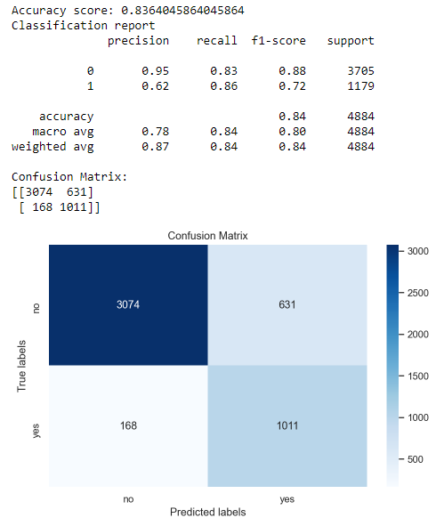
Confusion Matrix (Image by Author)

Step 7) Predict test data

• After tuning, the AUC score increased from 92.69% to 92.90%

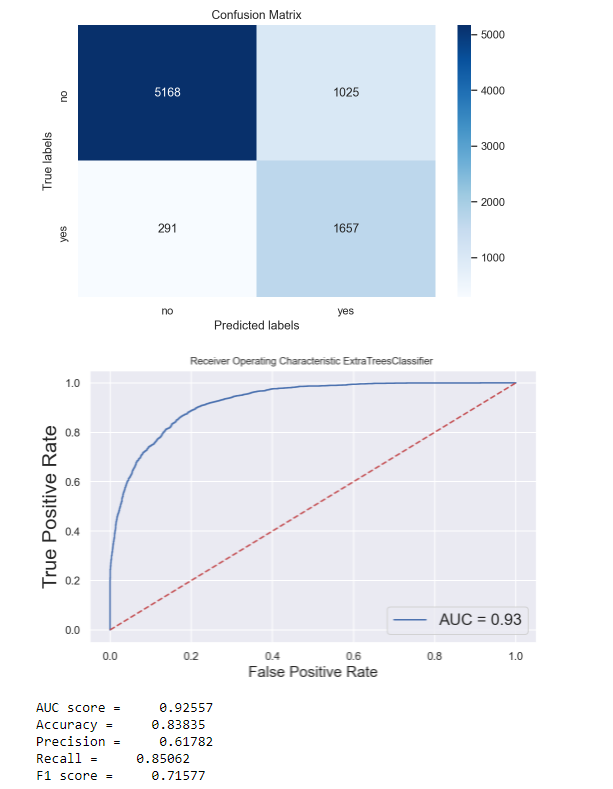
Prediction result (Image by Author)

• The key indicator must depend on project’s goal. However, we should compare train and test results. (Select AUC for this project)
  – AUC score = 92.56% (model = 92.90%)
  – Accuracy = 83.84% (model = 83.54%)
  – Precision = 61.78% (test_model = 61.38%)
  – Recall = 85.06% (test_model = 85.78%)
  – F1 score = 71.58% (test_model = 71.55%)
  – Type I error_per_Total = 12.59% (test_model = 12.92%)
  – Type II error_per_Total = 3.57% (test_model = 3.44%)

Note:
- Type I error → (Real = Class_0, Predict = Class_1) = 291/8141
- Type II error → (Real = Class_1, Predict = Class_0) = 1025/8141

---

Please feel free to contact me, I am willing to share and exchange on topics related to Data Science and Supply Chain. Facebook: facebook.com/nattapong.thanngam
Linkedin: linkedin.com/in/nattapong-thanngam